Multiple Testing, an overview of different decision rules
Hypothesis testing is a very useful tool in statistics. It helps draw conclusions about a population using sample data. Much of the emphasis in classical statistics focuses on testing a single null hypothesis. In other words, the basic framework usually compares two mutually exclusive statements about the population to determine which one is best supported by the sample data. Here we go one step ahead, and we face the contemporary challenge of testing a large number of hypotheses, as often needed in the era of big data.

In the first section, we will provide a brief review of null hypotheses, p-values, and other key ideas of hypothesis testing. However, we assume that the reader has had some previous exposure to these topics. If you are not familiar with these concepts yet, I recommend you this article, it is an excellent introduction. In the remainder of this post, we will explore different methods for effective multiple testing, and we will discuss their pros and cons.
Elements of hypothesis testing
The pipeline for the single hypothesis testing can be summarised as follows.
- Formulating the null and alternative hypotheses. For example, if we are considering a linear regression that tries to infer the value of a response variable y based on a set of predictors x, we could be interested in testing the null hypothesis “the coefficient for the first predictor is zero” against the (mutually exclusive) alternative hypothesis “the coefficient for the first predictor is different from zero”.
- Constructing the test statistic. The test statistic depends on the situation we are studying, and it is a measure of evidence against the null hypothesis.
- The realization of the test statistic is then used to compute the p-value, i.e. the probability of observing something at least as extreme, under the assumption that the null hypothesis is true. In other words, small p-values suggest that the null hypothesis should be rejected (because otherwise, it would be unlikely to observe such a value for the test statistic).
- But what is a small p-value? This question can only be answered heuristically, and in general, we need to pick a procedure that maps the p-value to the final decision, whether to believe in the null hypothesis or in the alternative hypothesis. An example could be rejecting the null hypothesis if the p-value is less than 0.05.

The described pipeline is inherently probabilistic and prone to errors. The possible outcomes after our decision are shown in the following table.

Now a fundamental observation. Hypothesis testing has two main goals:
- Making discoveries, i.e. rejecting the null hypothesis. This justifies the definition of power as the probability of correct inference, under the assumption that the alternative hypothesis holds.
- Minimizing the number of false discoveries, i.e. having a small probability for type I errors.
In other words, we want to contain the probability of a type I error below a certain threshold α, and at the same time, we aim for large power. Of course, we also aim at containing the type II errors, but a small probability for type I errors is more important, as those kinds of errors are often more costly.
For the single hypothesis testing, we can use the following simple procedure: if the p-value is less equal than α, then we reject the null hypothesis. Otherwise, we fail to reject the null hypothesis. In this case, using the uniformity of p-value, we get:

In the upcoming sections, we will explore different decision rules that are more appropriate in the context of multiple testing. But before doing it we still need to… define multiple testing and explain why it is interesting.
Multiple testing and its challenges
In the previous section, we saw that for the classical case, rejecting the null hypothesis if the p-value is below α provides a simple way to control the type I error at level α: if the null hypothesis is true, then there is no more than a probability of α that we will reject it.
But now imagine the following scenario: we are testing a new drug and we want to test, whether it has an effect on (a subset of) m different symptoms. In this context, it is natural to consider the following null/ alternative hypotheses.

As in the single hypothesis testing, we get a list of m p-values, one for each symptom. Now the main question is: given the m p-values, how do we decide which null hypotheses to reject and which ones not?
The first (naive) idea is to do the same thing we did for the single hypothesis testing: rejecting the i-th null hypothesis if its p-value is below the threshold α. To see whether it is a good idea or not, we start by computing the probability of making at least one error of type I. Under the assumption of independent p-values we get:

Which is close to one for m large enough. This illustrates the main challenge of multiple testing: when testing a large number of hypotheses, we are bound to get some very small p-values by chance. If we make a decision about whether to reject each null hypothesis without accounting for the fact that we have performed a large number of tests, then we may end up rejecting a great number of true null hypotheses, i.e. making a large number of type I errors. This is not desirable, as it contrasts with one of our goals for hypothesis testing.
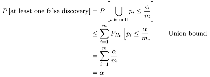
To improve this, we could be more conservative: instead of rejecting the i-th null hypothesis when its p-value is less than α, we could pick a smaller threshold, for instance α/m. Then we would have:

Which achieves our second goal. This decision rule is known as Bonferroni Method and, apart from achieving one of the goals of hypothesis testing, it has the further advantage of having a number of desirable properties that make it useful to obtain confidence intervals. However, it has one major drawback: it will only reject the null hypothesis when the corresponding p-value is very small, i.e. when it is very confident of the decision. For this reason, the method has the drawback of being too conservative, of having low power. This is in contrast to the first goal of hypothesis testing: making discoveries. Now the natural question is: can we do achieve the best of both worlds? Can we find a method that has higher power, but still a small probability for type I errors?
A (first) improvement towards a solution is given by the following algorithm, known as the Bonferroni-Holmes Method.
Bonferroni-Holmes Method
The Bonferroni-Holmes Method improves the Bonferroni Method by keeping the probability of false discoveries below the threshold α, but it is less conservative and hence it makes more discoveries. The framework is described below.

We observe that the used thresholds are greater (equal) than the ones used in the Bonferroni Method. For this reason, we have higher power and we can make more discoveries.
But what is the probability of making false discoveries? Despite the less conservative thresholds, the computations below show that this probability is still upper bounded by α. In the proof, we denote with r the rank of the null hypothesis with the smallest p-value. In other words, after having sorted the p-values ascendingly, we pick the position of the smallest p-value, where the null hypothesis holds.

We have now discussed two methods to contain the probability of making false discoveries below a threshold α. But is this the best approach? After all, to make the probability of false discovery small, a method that accepts all the null hypotheses would make the perfect job! However, it would be completely useless since it contrasts our main goal of making (right) discoveries. This observation motivates the following method, known as Benjamini-Hochberg Procedure.
Benjamini-Hochberg Procedure
Before diving into the method, we need to introduce a bit of notation. It is convenient to classify the m hypotheses we are testing as follows.

Where we denote with V, S, R, U, W, m-R, … the number of occurrences in the respective categories.
Until now we focused on containing in guaranteeing P[V≥1]⩽ α. This measure is known as family-wise error rate, or FWER for short. As mentioned before, it would be trivial to achieve an FWER of zero, by simply accepting all null hypotheses. This justifies the introduction of a new metric. For example, we could try to make sure that the ratio of false positives (V) to total positives (V+S=R) is sufficiently low. This metric is called false discovery proportion, and it is formally defined below.

It might be tempting to control the false discovery proportion directly, but unfortunately, it is not possible, since we don’t know the ground truth on any particular dataset. Therefore, we instead control the false discovery rate (FDR), which is defined as the expectation of the false discovery proportion. In other words, FDR=E[False discovery proportion]=E[V/R]. Optimizing the FDR is particularly convenient because it leads to decisions with higher power than Bonferroni(-Holmes).
We now dive into the Benjamini-Hochberg procedure that, given the p-values corresponding to the m hypotheses that we want to test, provides a decision rule with an FDR upper bounded by α.

We illustrate an intuition on why the Benjamin-Hochberg procedure contains the FDR below a threshold. First, we define the following two sets

and then we get

Note that the “proof” above is not entirely correct because we assumed that R is not random, which is not the case. Since the formal proof is quite involved and we think it does not bring much additional value, we refrain to report it here, and we refer the interested reader to the original paper.
Conclusion
In this post, we discussed three methods to extend the single hypothesis testing framework to multiple hypotheses. We started with the simple Bonferroni Method and with its improved version, the Bonferroni-Holmes Method. Both procedures control the FWER for m null hypotheses at level α. The former uses a constant threshold, the second an adaptive threshold that is independent from the data. We then discussed the limitations of controlling the FWER and we introduced the FDR, which can be controlled with the more involved Benjamini-Hochberg procedure, which chooses the p-values based on the data. The advantage of the Benjamini-Hochberg procedure is that it allows having high power (first goal of hypothesis testing), without a small probability for type I errors (second goal of hypothesis testing). The Benjamini-Hochberg procedure has been around since the mid ’90s. While a great many papers have been published since then proposing alternative approaches for FDR control that can perform better in particular scenarios, the Benjamini-Hochberg procedure remains a very useful and widely-applicable approach.
References
[1] G. James, D. Witten, T. Hastie, R. Tibshirani, An Introduction to Statistical Learning with Applications in R, Second Edition, 2021
