GLUE, an application of (Graph) Variational Autoencoders in Computational Biomedicine

Multi-omics integration is a central topic in Computational Biomedicine, offering a unique opportunity to unveil the underlying functionalities of different cells. Most of the available single-cell technologies detect one modality per cell only: for instance, to detect chromatin accessibility we need single-cell ATAC-sequencing, while we perform single-cell RNA sequencing to get the transcriptome.

Source: https://www.illumina.com/

Given the plethora of existing sequencing methods, it is easy to obtain unpaired data from different “omics”. However, to fully exploit their potential, computational integration is essential. A major obstacle in integrating unpaired multi-omics data is that different omic layers typically have distinct feature spaces. Ideally, we would like to combine data from different omics in a common embedding space that satisfies the following properties:

1. The embedding space has reasonable dimensionality. We often want to perform dimensionality reduction to avoid undesirable phenomena arising in high dimensions.
2. Different omics are aligned in the embedding space. They should be well-mixed such that a discriminator is not able to determine what original omic generated the embedding.
3. The cell embeddings faithfully conserve their biological variation. If two original features are related (in terms of regulatory interaction), their embeddings should be “similar”.

In this post, we describe GLUE [1](graph-linked unified embedding): a framework that proposes a combination of (graph) variational autoencoders for effective multi-omics integration.

In the next section, we provide an overview of the model, where we also provide intuitions on how the different components contribute to accomplishing the goals above. Afterward, we introduce the math behind GLUE (in this post we sketch the main ideas, for more details check out here). The paper presents a number of examples where GLUE shines. They are very interesting, but we refrain to discuss them here. The goal of this post is giving a brief (engineering-oriented) overview of the model, not diving into the biomedical technicalities.

Overview of the Model

Let’s consider K omic layers (in the figure below, we would have K=3). The model’s input is the following.

• Cell data for each omic layer. Note that, in general, it is possible to have a different number of cells for different layers. Moreover, the feature spaces of different layers can have different dimensionality.
• A knowledge-based graph (called guidance graph), that models prior knowledge about cross-layers regulatory interactions. The vertices in the graph are the features of the input layers, and an edge (u, v) represents a signed regulatory interaction from feature u (of a certain layer) to feature v (of another layer).

The goal is to compute a common m-dimensional embedding for the multi-omics features satisfying the goals listed in the introduction. In particular, m should be small enough to satisfy goal (1). Moreover, since the prior knowledge in the guidance graph is not perfect and might contain errors, we want the embeddings to be robust to small perturbations in the guidance graph.

Graphically, GLUE looks as follows.

Overview of GLUE (source)

Given the high modularity of the model, we start with a brief high-level description of the components.

• A graph variational autoencoder [2] compresses the guidance graph. More specifically, we want to compress its adjacency matrix such that the number of rows does not change, but the number of columns is reduced to m (note that this is the same dimensionality as the output embedding).
• K variational autoencoders (one for each omic layer). Each autoencoder is trained to minimize its reconstruction loss. However, there are two subtle differences with canonical variational autoencoders. First: to reconstruct the input, the decoder does not only use data from the autoencoder embedding, but also from the embedding of the guidance graph. This is crucial towards achieving goal (3). In fact, without properly linking the components, the K variational autoencoders would be parametrized independently, leading to inconsistent semantics between different omics. Second: the decoder is not a neural network, but a simple linear mapping. This choice was made possible by the fact that the non-linear encoders are good enough to properly align modalities, and a non-linear decoder has the desirable property of ensuring interpretability to the embedding spaces.
• A discriminator D that receives an embedding as input, and outputs a K-dimensional softmax output. Its goal is assigning an embedding to the omic layer that generated it. D is trained with an adversarial strategy similar to GANs. As a notable result from game theory, the discriminator will be fooled, and hence this strategy leads to a proper alignment between different omic layers, satisfying goal (2).

Derivation of the objective function

The goal is finding the “best” embedding or, more precisely, the probability of the embeddings given the inputs. Formally, for each omic layer, we would like to estimate the following distribution.

The expression above, unfortunately, is computationally intractable because of the integral in the denominator. For this reason, instead of computing the probability directly, we use two neural networks (the data encoders) to get the following approximate distribution.

Note that the equality holds because the encoders of the omic layers and the graph variational autoencoder are independent.

But how should the neural networks be trained? Recall that we want them to approximate the original (intractable) distribution, so it is natural to introduce the following objective function.

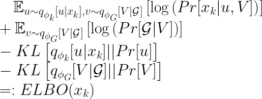
We omit the details here (please refer to the additional material), but it can be shown that this is equivalent to maximizing the following evidence lower bound (aka ELBO).

The intuition of the ELBO is that we aim to find embeddings with a similar distribution to the priors, and that at the same time allow a high-quality reconstruction of the input.

From the architecture’s description and the design choices discussed in the previous section, we can infer the following (conditional) independencies.

• The encoders are all independent.
• The priors of the omic embeddings and the graph embedding are independent.
• The graph decoder uses only the graph embedding, while the omic decoders use both their embedding and the graph embedding.

These observations are particulary useful to further simplify the ELBO. We get:

Until now we described the objective function for a single embedding. From the formula above, it is clear that we have two encoders (one for the omic features, one for the graph embedding). But where does the decoder comes into play? The answer is short: the decoders are used in the formula above to compute the conditional probabilities of the observations given the embeddings. What deserves more words are some insights about the author’s choices for the decoders. For the conditional probability of the omic features, a simple linear mapping and some probability distribution is used. The paper proposes the negative binomial distribution, but other solutions can be explored. For the graph decoder, no parameter needs to be learned, as a simple MLE is used. We refrain from giving the details here, but the idea is that the probability of having an edge between two nodes with “similar” embeddings is high, and it decreases with a larger “distance” between the two embeddings. The “similarity” of the embeddings is proportional to their scalar product. This is coherent with goal (3) from the introduction.

Note that, until now, we only focused on the objective derivation for the graph autoencoder and a single omic layer. To combine all the omic encoders, we optimize the following.

Where Θ is the parameter space of the omic decoders. The objective function above can be further rearranged. We get:

where

and

Finally, we are (almost) there! We derived a loss function to find encoders/ decoders that are trained to:

• Correctly reconstruct the input from the embeddings.
• Compute embeddings as close as possible to their priors (in order to avoid collapse to a single magnitude).
• Ensure that similar cells have similar embeddings. This is obtained thanks to the prior knowledge integrated with the guidance graph, and it helps towards achieving goal (3).

The last step that we perform ensures that different omics are aligned in the embedding space. In other words, we need a last step to achieve goal (2). We hence introduce a decoder trained in an adversarial fashion. The decoder’s goal is to correctly assign each omics embedding to the omic layer that generated it. Formally, we want to minimize the following quantity.

Wrapping up, the objective function of GLUE is given by

where we introduced two hyperparameters to control the contributions of alignment and graph-based feature embedding, i.e. a trade-off between goal (2) and goal (3).

Conclusion

In this post, we derived the objective function of GLUE, a scalable algorithm that performs high quality multi-omics integration. We neglected many interesting aspects of GLUE, both on the biomedical side (the paper presents a number of success stories), and also on the computational side. For example, we omit how the objective function can be optimized (in a nutshell, we use a reparametrization trick and gradient descent like algorithms), and also how to validate the model. However, we think that the derivation of the objective function is the most interesting part, as it provides many intuitions on what we should aim for when designing an algorithm towards multi-omics integration.

Bibliography

[1] Zhi-Jie Cao & Ce Gao, Multi-omics single-cell data integration and regulatory inference with graph-linked embedding, 2022.

[2] An introduction to Graph Variational Autoencoders from Towards Data Science: https://towardsdatascience.com/tutorial-on-variational-graph-auto-encoders-da9333281129